How To Create A Bell Curve In Excel With Data

Excel Bell Curve (Table of Contents)

• Bell Curve in Excel
• How to Make a Bell Curve in Excel?

Bell Curve in Excel

Bell curve in excel is mostly used in the Employee Performance Appraisal or during Grading of the Exam Evaluation. The Bell curve is also known as the Normal Distribution Curve. The main idea behind the bell curve is when everybody in the team or class is a good performer, how will you identify who is the best performer, who is the average performer and who is the poor performer in the team or class.

So before we proceed further, let us first understand the concept of the Bell Curve in Excel with the help of a simple example.

Suppose there are 100 students in a class who appeared for the exam, as per the education system, whoever gets more than 80 will get an A grade. But then there will be no difference between a student who scores 99 and a student who scores 81 as both would get an A grade.

Using the Bell curve approach, we can convert the marks of the students into Percentile and then compare them with each other. Students getting lower marks will be on the left side of the curve, and students getting higher marks will be on the right side of the curve, and most of the students who are average will be in the middle of the curve.

We need to understand two concepts to understand this theory better.

1. Mean – It is the average value of all Data Points.
2. Standard Deviation – It shows how much Dataset varies from the Mean of the Dataset.

How to Make a Bell Curve in Excel?

To make a bell curve in Excel is very simple and easy. Let's understand how to make a bell curve in excel with some examples.

You can download this Bell Curve Excel Template here – Bell Curve Excel Template

Example #1

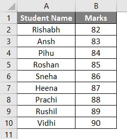
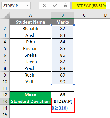
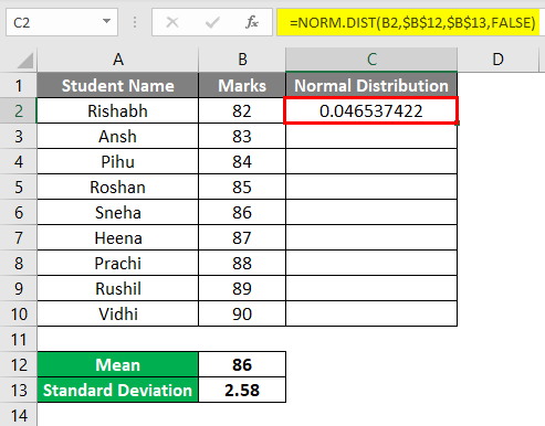
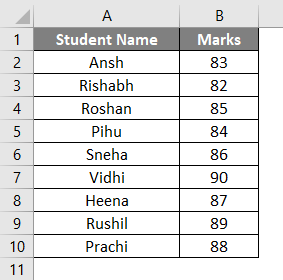
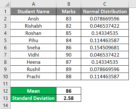
Suppose there are 10 students in a class who has got the below marks out of 100.

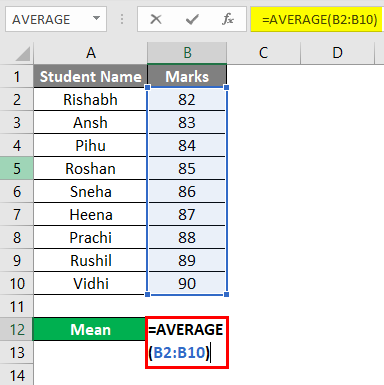
You can calculate the Mean with the help of the Average Function.

In cell B12, I have inserted the Average Function, as you can see in the below screenshot.

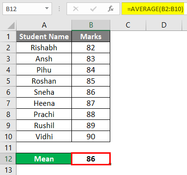
The result of the Average Function is 86. So we can say that the Mean in our example is 86, which will be the center of the Bell curve.

Now we need to calculate the Standard Deviation, which we can do with the help of the STDEV.P function.

So the result of the standard deviation in our case is 2.58.

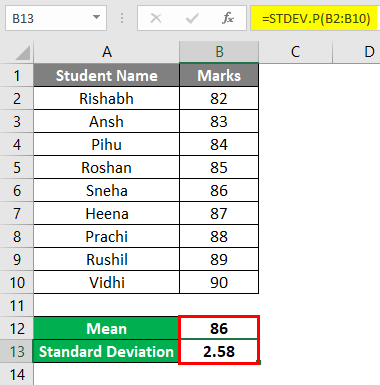
In this case, the value of 2.58 means that most of the students will be in the range of 86-2.58 or 86+2.08.

Now to calculate the normal distribution, you need to insert the formula for normal distribution in the next cell of Marks. The syntax of the formula is as below.

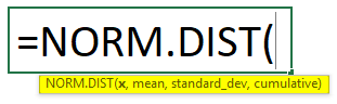
So let us insert the formula from cell C2. Please make sure that you freeze the cells for Mean and standard deviation in the formula.

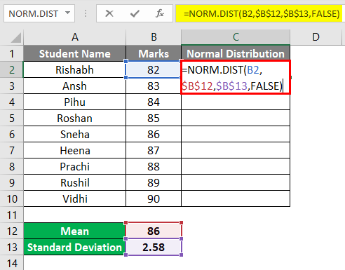
The Result is given below.

Now drag the formula in the below cells till cell C10.

Insert a Bell Curve in Excel (Normal Distribution Curve)

Now, as all the data is ready with us for the Bell curve, we can insert a Bell curve chart in excel.

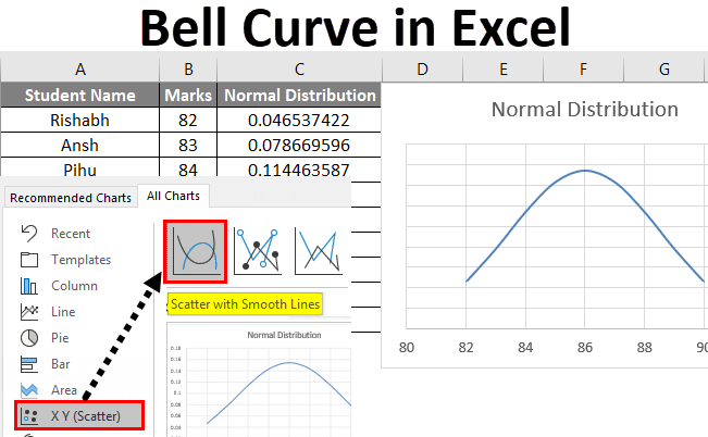
First, select the Marks of all student and the Normal Distribution column, which we calculated above, and under the Insert tab, click on Recommended Charts as shown below.

Now under the Recommended chart, you will see lots of option for different types of charts. But to get a normal distribution curve (Bell Curve), follow the below steps.

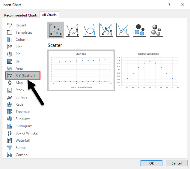
• First, click on All Charts.

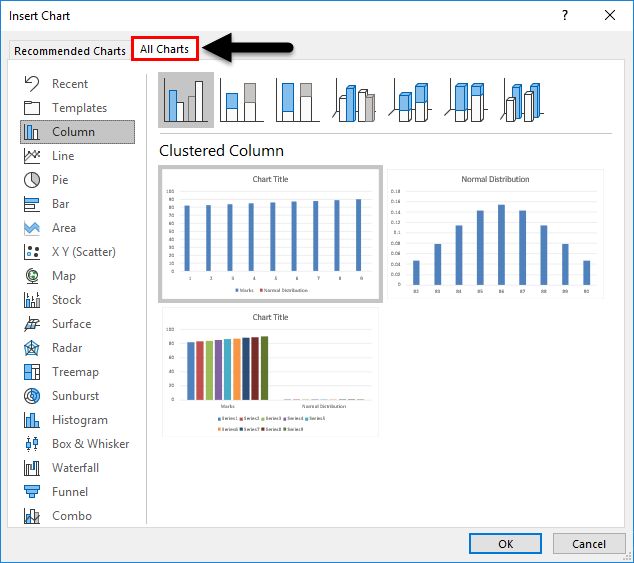
• Now select XY Scatter Chart Category on the left side.

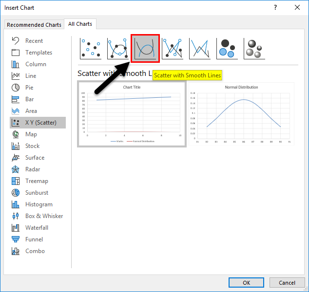
• You can see the built-in styles at the top of the dialog box; click on the third style, Scatter with Smooth Lines.

• Select the Second chart and click on Ok.

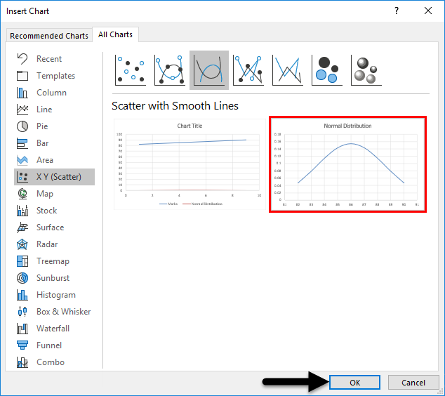
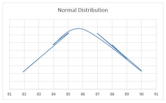
• So now you will be able to see the Bell curve in your excel sheet as below.

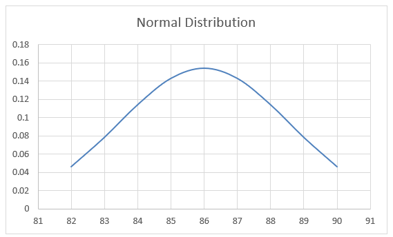
Now when you look at the Bell Curve, you can see that the maximum number of student will be in the range of 83.42 & 88.58(86-2.58 =83.42 & 86+2.58 = 88.58).

In our example, there are 6 students who are in between 83 & 88. So I can say that they are the average performers in the class. Only 2 students have scored more than 88,, so they are the best performers in the class. Only one student has scored below 83, so he is a poor performer in the class.

Remove the Vertical axis from the graph.

The Horizontal axis is the Marks scored, and the Vertical axis is the Normal Distribution. If you do not want to see the Vertical axis of Normal Distribution, you just need to follow the below steps.

• Click on the graph, and you will see the "+" sign on the right corner of the graph area.

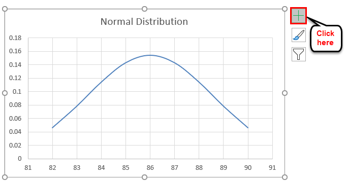
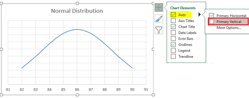
• After clicking on the + sign, you will see an option for Axis as below. Click on the Axis button, and you will see two options for Horizontal Axis and Vertical Axis. Just uncheck the Vertical Axis.

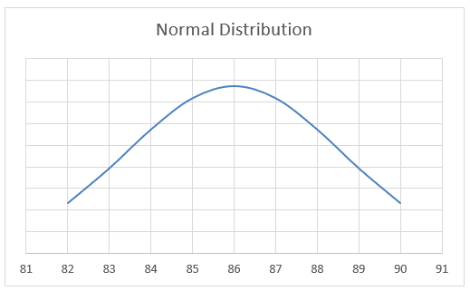
• This Bell curve helps you identify who the top performer in your team is and who is the lowest performer and help you decide the ratings of the employee.

When Data is not sorted in Ascending Order

So in the above example, Marks were sorted in ascending order, but what if the data is not arranged in the ascending order. Then we will not be able to get a smooth bell curve as above. So it is very important to arrange the data in ascending order to get a smooth bell curve in excel.

Example #2

Let's take a similar example, but data will not be sorted in ascending order this time.

The Average (which is Mean), Standard Deviation and Normal Distribution will all remain the same.

But the Bell curve graph of the same example will look different because Marks were not sorted in the Ascending order. The Bell curve graph will now look as below.

So as you can see in the graph, it started with 83 and ends with 88. Also, you can notice that the graph is not as smooth as it was in example 1. So to get a smooth Bell curve in excel, it is very important to sort the data in ascending order.

Things to Remember

• Always make sure to sort the data in Ascending order to get a smooth bell curve in Excel.
• Remember to Freeze the Cell of Average (Mean) & Standard Deviation when inputting the formula for the Normal Distribution.
• There are two formulas for Standard Deviation – STDEV.P & STDEV.S (P stands for Population & S stands for Sample). So when you are working on Sample data, you need to use STDEV.S.

Recommended Articles

This has been a guide to Bell Curve in Excel. Here we discuss how to make a Bell Curve in Excel along with excel examples and a downloadable excel template. You can also go through our other suggested articles –

1. Scatter Chart in Excel
2. Scatter Plot Chart in Excel
3. Combination Charts in Excel
4. Stacked Area Chart

How To Create A Bell Curve In Excel With Data

Source: https://www.educba.com/bell-curve-in-excel/

Posted by: ferrarogreggelf44.blogspot.com

Share this post